Deep Learning: Recurrent Batch Normalization
These are my study notes on Recurrent Batch Normalization as preparation for the Deep Learning Study Group (SF) session on April 26, 2016. These notes also contain some info from Batch Normalization: Accelerating Deep Network Training by Reducing Internal Covariate Shift.
Recurrent Neural Networks, or RNNs, work great for many tasks. A big downside is that training these deep networks takes a significant amount of time. One effect that causes RNNs (and other deep neural nets) to require long training time is called internal covariate shift.
Internal Covariate Shift
In a neural network, the output of one layer is input to the next layer. Let’s think of one layer deep in the network. There are many layers preceding this one layer, each of which has an influence on what input this layer will see. When you are just starting to train your network, the distribution of the input data to this layer sees will vary significantly over time. The change of the distribution of the input data to a layer during training is called internal covariate shift. It is a challenge to pick a learning rate, parameter initialization, and activation function that allows a deep net to converge (i.e. learn anything) under these challenging conditions, and is a topic that many deep learning papers have focused on.
Solution: Batch Normalization
The purpose of batch normalization is to help minimize the difficulties caused by internal covariate shift. We normalize the input to each layer by adjusting the mean and variance of the input across one minibatch. This avoids the shift of input distribution over time, and gives the optimization one less problem to worry about (i.e. we have a better ‘conditioned’ optimization). Batch normalization works great when used in convolutional neural nets. It speeds up training by a large margin and achieves top performance on rankings such as CIFAR. Let’s take a look at the definition:
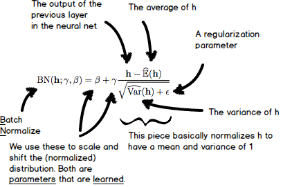
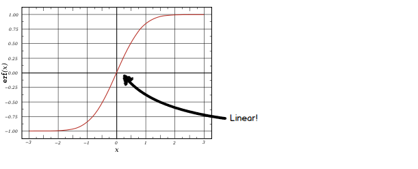
The division at the end of the equation above normalizes the values in the vector \( h \) to a mean of 0 and standard deviation of 1. We then scale the values using the vector \( \gamma \), and shift them using the vector \( \beta \). That seems odd at first, but there is a very good reason for doing so. Many activation functions, such as the sigmoid and tanh functions, are linear around 0. It would be silly to always normalize your inputs to mean 0 and stdev 1; the net would act as if it doesn’t have any nonlinearities and would lose the ability to learn the generalizations neural networks are known for!
Batch Normalization and RNNs
The purpose of this paper is to show how to effectively use batch normalization in RNNs. Now that we know how batch normalization works, let’s see how it’s used in a LSTM network:
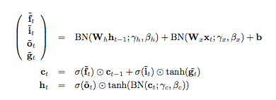
Ok, batch normalization is applied to the state of the previous timestep of the RNN (\( W_h h_{t-1} \)), the input vector (\( W_x x_t \)) and the memory cell state (\( c_t \)). Note that the update of cell \( c_t \) does not use batch normalization: the purpose of the memory cell in an LSTM is to avoid a vanishing gradient (which is an effect that causes the gradient to become very weak during backpropagation through many layers). The authors mention that batch normalization on \( c_t \) would alter the gradient flow and affect the dynamics of the LSTM.
Looking back at the definition of batch normalization, there are a few interesting things to note. First, the dimension of \( h \) is \( \mathbb{R}^{d}\), so we are looking at the activations during one timestep for one sample. The dimensions of \( \widehat{\mathbb{E}}(h) \) and \( \widehat{var}(h) \) must also be \( \mathbb{R}^{d}\). Now here’s the important part: the values of \( \widehat{\mathbb{E}}(h) \) and \( \widehat{var}(h) \) are the average and variance of the values of the vector \( h \) in the current minibatch for the current timestep. That means that we are independently normalizing each value in the vector \( h \) based on all \( h \) vectors in the current minibatch, and do so independently for every timestep. This turns out to be important.
The reason the normalization is done independently for every time step is that the variance and mean of the inputs go all over the place during the first few timesteps (see Figure 1 of the paper). Notice also how the mean and variance don’t really change anymore after 10 timesteps or so - we’ll get back to that later.
Key point: Initialization of Gamma
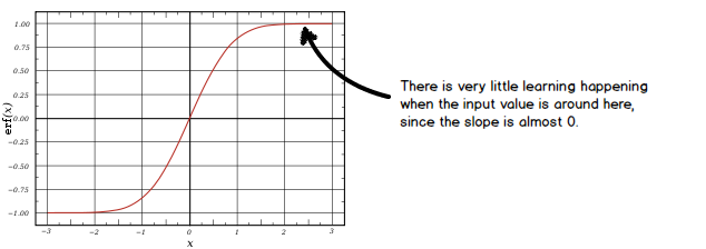
Before this paper was published, batch normalization had not worked well for RNNs. The authors figured out that this is caused by the initialization of \( \gamma \). Remember that \( \gamma \) determines the standard deviation of the input to a layer. When its value is set to something too high, we could quickly cause the tanh function to saturate. When the tanh is saturated, it effectively stops learning:
Questions from the meetup: Why not swap tanh with another activation function that avoids saturation (such as leaky ReLU)? Why not use gradient clipping to avoid saturation?
It turns out that everything works great when \( \gamma \) is initialized to 0.1.
Testing Time
So far batch normalization has helped train the RNN faster by reducing internal covariance shift. We do still have to apply this normalization during testing. For testing, the values of \( \widehat{\mathbb{E}}(h) \) and \( \widehat{var}(h) \) are calculated based on the entire training set.
Remember how the mean and variance of the input don’t really change much after 10 timesteps or so? And that \( \widehat{\mathbb{E}}(h) \) and \( \widehat{var}(h) \) are different for every time step? Just use the same values for \( \widehat{\mathbb{E}}(h) \) and \( \widehat{var}(h) \) after the nth timestep to generalize to any amount of timesteps necessary during testing.